Introduction
![The pcDuino board]()
The beauty of the pcDuino lies in its extraordinarily well exposed hardware peripherals. However, using these peripherals is more complex than using them on, say, an Arduino-compatible board.
This tutorial will help you sort out the various peripherals, what they can do, and how to use them.
Before we get started, there are a few things you should be certain you’re familiar with, to get the most out of this tutorial:
- pcDuino– some familiarity with the basics of the pcDuino is needed before you jump into this. Please review our Getting Started with pcDuino tutorial before going any further.
- Linux – the biggest thing you should be familiar with it the Linux OS. Remember, pcDuino is not an Arduino—it is a modern microcomputer running a fully-functional, if compact, operating system.
- SPI– a synchronous (clocked) serial peripheral interface used for communications between chips at a board level. Requires a minimum of four wires (clock, master-out-slave-in data, master-in-slave-out data, and slave chip select), and each additional chip added to the bus requires one extra chip select line.
- I2C– also known as IIC (inter-integrated circuit), SMBus, or TWI (two-wire interface), I2C uses only two wires (bidirectional data and clock lines) to communicate with multiple devices.
- Serial Communication– an asynchronous (no transmitted clock) data interface with at least two wires (data transmit and data receive; sometimes, additional signals are added to indicate when a device is ready to send or receive).
- Pulse Width Modulation– a digital-to-analog conversion technique using a fixed frequency square wave of varying duty cycle, which can be easily converted to an analog signal between 0V and the full amplitude of the digital IC driving the signal.
- Analog-to-Digital Conversion– measurement of an analog voltage and conversion of that voltage into a digital value.
All of the code in this tutorial can be found online, in our pcDuino Github repository. It’s not a bad idea to check there for any updates to the code since this tutorial was written.
Your First Program
Even if you’ve programmed Linux computers before, it may be a good idea to give this section a brief run-through, just to make sure you know what to do for this particular device. If you’ve never written any code for anything more advanced than an Arduino, that’s okay, too! We’ll get you started.
This tutorial is going to cover two different languages: Python 2.7 and C++. It is not meant to be a “learn to program” tutorial; rather, it’s meant to introduce and provide examples for accessing the various resources on the pcDuino, as well as getting code to compile and run.
C++ Programming
Compiling and running a C++ program is pretty easy. All you need to do is invoke the g++ compiler pointed at a source file and it will build an executable of that file.
Let’s give it a try. Open a new LeafPad document and type in this code:
language:cpp
#include <stdio.h> // Include the standard IO library.

int main(void) // For C++, main *must* return type int!
{
  printf("Hello, world!\n"); // Print "Hello, world!" string to the command line.
}
Save the file with the name “hello_world.cpp” to any convenient directory (say, “~/Documents”), then open an LXTerm window and navigate to that directory. At the command prompt, type these commands:
language:text
g++ hello_world.cpp -o hello_world
./hello_world
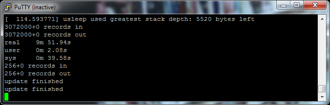
Here’s what your command line output should look like (note that, for most examples in this tutorial, I’m running the commands in a PuTTY terminal on Windows, to make my life a little easier—that’s why the menu bar looks different to LXTerm):
![Hello world C++ output]()
So, there you have it: your first C++ program written and run on the pcDuino!
Python Programming
Python programming is even easier than C++. Python is an interpreted language, which means that there’s no compilation step which produces an executable. The code you write gets executed line-by-line by the interpreter. There’s a price to pay in terms of performance, in most cases, but the ease of coding in Python, coupled with incredibly powerful libraries, makes it very attractive.
Open another Leafpad document and put this code in:
language:python
print "Hello, world!"
That’s it. Simple, innit? Now, save that file to a convenient location as “hello_world.py”, and get an LXTerm prompt in that directory. Type in the following command:
language:text
python hello_world.py
Your output should look a lot like this:
![Hello world Python output]()
And that’s Python. If you haven’t used Python before, I strongly suggest you give it a try—it’s insanely powerful. All of the examples in this tutorial will be done in both C++ and Python; it will quickly become obvious why Python is a favorite for getting good results, fast.
Accessing GPIO Pins
The pcDuino comes with 18 pins that can be accessed as, among other things, general purpose I/O.
Hardware
Accessing GPIO pins is not hard; simply open the file associated with the pin you wish to access and read or write that file. The files are located in the following locations:
language:text
/sys/devices/virtual/misc/gpio/mode/
/sys/devices/virtual/misc/gpio/pin/
Each pin has its own file. Note that there are 20 files; only 18 of them are actually mapped to available pins. The files map to the pins as seen in the image below:
![GPIO pin mapping on the pcDuino]()
Some pins can do double (or triple) duty. Writing certain strings to the “mode” file will activate the various different modes (serial, SPI, input, output, etc) for the particular pin you’re accessing; we’ll cover those different values in later exercises. For now, you really only need to worry about three of them:
- ‘0’ – make the pin an INPUT
- ‘1’ – make the pin an OUTPUT
- ‘8’ – make the pin an INPUT, with a pull-up resistor
The logic on these pins is 3.3V; attempting to use 5V devices can cause damage to your pcDuino. The output current capacity is not as high as it is on Arduino-type boards, but should be sufficient to drive a small LED fairly easily.
GPIO in C++
Here is an example program for using C++ to read and write GPIO pins. It’s pretty simple: it waits for a button attached to GPIO2 to be pressed (thereby pulling the pin low), then turns LEDs attached to the various GPIO pins on one at a time, then back off again.
language:cpp
#include <fcntl.h>
#include <stdio.h>
#include <string.h>
#include <unistd.h>

#include "gpio_test.h"

// These arrays will become file descriptors for the 18 IO pin and mode files.
int pinMode[18];
int pinData[18];

int main(void)
{
  int i = 0;       // Loop iterator

  char inputBuffer = HIGH; // create and clear a buffer for data from pins

  char path[256]; // nice, long buffer to hold the path name for pin access

  // This first loop does four things:
  //   - initialize the file descriptors for the pin mode files
  //   - initialize the file descriptors for the pin data files
  //   - make the pins outputs
  //   - set all the pins low
  for (i = 2; i <= 17; i++)
  {
    // Clear the path variable...
    memset(path,0,sizeof(path));
    // ...then assemble the path variable for the current pin mode file...
    sprintf(path, "%s%s%d", GPIO_MODE_PATH, GPIO_FILENAME, i);
    // ...and create a file descriptor...
    pinMode[i] = open(path, O_RDWR);
    // ...then rinse, repeat, for the pin data files.
    memset(path,0,sizeof(path));
    sprintf(path, "%s%s%d", GPIO_PIN_PATH, GPIO_FILENAME, i);
    pinData[i] = open(path, O_RDWR);
    // Now that we have descriptors, make the pin an output, then set it low.
    setPinMode(pinMode[i], OUTPUT);
    setPin(pinData[i], LOW);
    printf("Pin %d low\n", i);  // Print info to the command line.
  }

  // Now, we're going to wait for a button connected to pin 2 to be pressed
  //  before moving on with our demo.
  setPinMode(pinMode[2], INPUT_PU);

  do
  {
    printf("Waiting for button press...\n");
    // This lseek() is very important- must read from the top of the file!
    lseek(pinData[2], 0, SEEK_SET);
    // Read one byte from the pinData register. The first byte will be '1' if
    //   the pin is high and '0' if it is low.
    read(pinData[2], &inputBuffer, 1);
    usleep(100000);       // Sleep for 1/10 second.
  } while (inputBuffer == HIGH);

  // After the button press, let's scan through and turn the lights on one
  //   at a time, the back off again. After that, we're done.
  for (i = 3; i <= 17; i++)
  {
    setPin(pinData[i], HIGH);
    printf("Pin %d HIGH\n", i);
    usleep(250000);
  }

  for (i = 17; i >=3; i--)
  {
    setPin(pinData[i], LOW);
    printf("Pin %d LOW\n", i);
    usleep(250000);
  }
}

// These two 'set' functions are just wrappers to the writeFile() function to
//   make the code prettier.
void setPinMode(int pinID, int mode)
{
  writeFile(pinID, mode);
}

void setPin(int pinID, int state)
{
  writeFile(pinID, state);
}

// While it seems okay to only *read* the first value from the file, you
//   seemingly must write four bytes to the file to get the I/O setting to
//   work properly. This function does that.
void writeFile(int fileID, int value)
{
  char buffer[4];  // A place to build our four-byte string.
  memset((void *)buffer, 0, sizeof(buffer)); // clear the buffer out.
  sprintf(buffer, "%c", value);
  lseek(fileID, 0, SEEK_SET);   // Make sure we're at the top of the file!
  write(fileID, buffer, sizeof(buffer));
}
GPIO Access in Python
Here’s the same program realized in Python. Again, it simply waits for a button on GPIO2 to be pressed, then scans through the other GPIO pins, making them first high, then low.
language:python
#!/usr/bin/env python

import time, os

## For simplicity's sake, we'll create a string for our paths.
GPIO_MODE_PATH= os.path.normpath('/sys/devices/virtual/misc/gpio/mode/')
GPIO_PIN_PATH=os.path.normpath('/sys/devices/virtual/misc/gpio/pin/')
GPIO_FILENAME="gpio"

## create a couple of empty arrays to store the pointers for our files
pinMode = []
pinData = []

## Create a few strings for file I/O equivalence
HIGH = "1"
LOW =  "0"
INPUT = "0"
OUTPUT = "1"
INPUT_PU = "8"

## First, populate the arrays with file objects that we can use later.
for i in range(0,18):
  pinMode.append(os.path.join(GPIO_MODE_PATH, 'gpio'+str(i)))
  pinData.append(os.path.join(GPIO_PIN_PATH, 'gpio'+str(i)))

## Now, let's make all the pins outputs...
for pin in pinMode:
  file = open(pin, 'r+')  ## open the file in r/w mode
  file.write(OUTPUT)      ## set the mode of the pin
  file.close()            ## IMPORTANT- must close file to make changes!

## ...and make them low.
for pin in pinData:
  file = open(pin, 'r+')
  file.write(LOW)
  file.close()

## Next, let's wait for a button press on pin 2.
file = open(pinMode[2], 'r+') ## accessing pin 2 mode file
file.write(INPUT_PU)          ## make the pin input with pull up
file.close()                  ## write the changes

temp = ['']   ## a string to store the value
file = open(pinData[2], 'r') ## open the file
temp[0] = file.read()       ## fetch the pin state

## Now, wait until the button gets pressed.
while '0' not in temp[0]:
  file.seek(0)      ## *MUST* be sure that we're at the start of the file!
  temp[0] = file.read()   ## fetch the pin state
  print "Waiting for button press..."
  time.sleep(.1)  ## sleep for 1/10 of a second.

file.close()  ## Make sure to close the file when you're done!

## Now, for the final trick, we're going to turn on all the pins, one at a
##   time, then turn them off again.
for i in range(3,17):
  file = open(pinData[i], 'r+')
  file.write(HIGH)
  file.close()
  time.sleep(.25)

for i in range(17,2, -1):
  file = open(pinData[i], 'r+')
  file.write(LOW)
  file.close()
  time.sleep(.25)
Unlike the Raspberry Pi, the pcDuino does have some analog input and output functionality. Here are examples of using the analog circuitry in your projects.
Hardware
![Analog pin mapping on the pcDuino]()
Analog output on the pcDuino is accomplished via PWM. There are six PWM enabled pins in the Arduino-ish headers: 3, 5, 6, 9, 10, and 11. These, of course, correspond to the PWM pins on Arduino boards. Pins 5 and 6 are true 520Hz 8-bit PWM; the others are limited to a range of 0-20 at 5Hz. The high-level output for all the pins is 3.3V.
Analog input on the pcDuino is done through six dedicated pins labeled A0-A5 on the Arduino-ish headers. A0 and A1 are six-bit inputs, returning a value from 0-63 over a range from 0-2V; A2-A5 are 12-bit inputs operating across the full 3.3V range. Setting an analog reference on the AREF pin is not supported as of the time of this writing.
Analog in C++
Analog input is handled through standard file stream input: simply open the appropriate file and read the value. Values are read as a string, so an atoi() conversion is necessary to get an integer value to work with.
Analog output is handled through a command line interface. Piping a value into a particular file via the system() call allows you to set the PWM level on the appropriate pins; file streams do not work for this. Again, the file expects a string, not an integer, so you must format the output appropriately.
This example program fades the PWM pins from off to on, slowly, then prints the output of each analog input.
language:cpp
#include <stdio.h>
#include <stdlib.h>
#include <string.h>
#include <fcntl.h>
#include <unistd.h>
#include "analog.h"

int adc[6];     // Array for file descriptors for the adc pins
int PWMMaxVal[6]; // Store the max values for the PWM outputs
char path[64];  // Nice big buffer for constructing file paths

int main(void)
{
  // For starters, let's create file descriptors for all the ADC pins. PWM is
  //   handled differently; see the analogWrite() function for details.
  for(int i = 0; i<= 5; i++)
  {
    memset(path, 0, sizeof(path));
    sprintf(path, "%s%s%d", ADC_IF_PATH, ADC_IF_FILE , i);
    adc[i] = open(path, O_RDONLY);
    memset(path, 0, sizeof(path));
    sprintf(path, "%s%s%d/%s", PWM_IF_PATH, PWM_IF_FILE , i, PWM_MAX);
    int PWMMaxFD = open(path, O_RDONLY);
    char PWMMaxStr[4];
    read(PWMMaxFD, PWMMaxStr, sizeof(PWMMaxStr));
    PWMMaxVal[i] = atoi(PWMMaxStr);
  }

  // Now, we'll blast all the PWM pins to zero.
  for(int j = 0; j<=5; j++)
  {
    analogWrite(j, 0);
  }

  // Now we can go about the business of dimming some LEDs.
  for(int j = 0; j<=5; j++)
  {
    for(int i = 0; i<=255; i++)
    {
      analogWrite(j, i);
      usleep(10000);
    }
    analogWrite(j, 0);
  }

  // Analog input is handled by file streams.
  for (int i = 0; i <= 5; i++)
  {
    char ADCBuffer[16];
    lseek(adc[i], 0, SEEK_SET);
    int res = read(adc[i], ADCBuffer, sizeof(ADCBuffer));
    int ADCResult = atoi(ADCBuffer);
    printf("ADC Channel: %d Value: %s", i, ADCBuffer);
  }
}

  // PWM pin access is handled by
  //   using the system() command to invoke the command process to execute a
  //   command. We assemble the command using sprintf()- the command takes
  //   the form
  //   echo <value> > /sys/class/leds/pwmX/brightness
  //   where <value> should be replaced by an integer from 0-255 and X should
  //   be replaced by an index value from 0-5
void analogWrite(int pin, int value)
{
  memset(path, 0, sizeof(path));
  value = (PWMMaxVal[pin] * value)/255;
  sprintf(path, "echo %d > %s%s%d/%s", value, PWM_IF_PATH, PWM_IF_FILE, \
    pin, PWM_IF);
  system(path);
}
Analog in Python
As usual, the Python code mirrors C++ functionally, but is somewhat simpler. The code performs a very similar operation to the C++ program—fade the PWM pins, then spit out the analog inputs.
language:python
#!/usr/bin/env python

import time, os

## For simplicity's sake, we'll create a strings and filenames for our paths
ADC_PATH= os.path.normpath('/proc/')
ADC_FILENAME = "adc"
PWM_PATH= os.path.normpath('/sys/class/leds/')
PWM_DIR = "pwm"
PWM_FILENAME = "brightness"
PWM_MAX = "max_brightness"

## create empty arrays to store the pointers for our files
adcFiles = []
pwmFiles = []
pwmMaxFiles = []

## create an empty array to store the maximum value for each channel of PWM
pwmMaxVal = []

## Populate the arrays with paths that we can use later.
for i in range(0,6):
  adcFiles.append(os.path.join(ADC_PATH, ADC_FILENAME+str(i)))
  pwmFiles.append(os.path.join(PWM_PATH, PWM_DIR+str(i), PWM_FILENAME))
  pwmMaxFiles.append(os.path.join(PWM_PATH, PWM_DIR+str(i), PWM_MAX))

## Now, let's scan the PWM directories and pull out the values we should use
##   for the maximum PWM level.
for file in pwmMaxFiles:
  fd = open(file, 'r')
  pwmMaxVal.append(int(fd.read(16)))
  fd.close()

## Let's dim some LEDs! The method for controlling a PWM pin on the pcDuino is
##   to send to the command interpreter (via os.system() this command:
##   echo <value> > /sys/class/leds/pwmX/brightness
##   where <value> varies from 0 to the maximum value found in the
##   max_brightness file, and X can be from 0-5.
for file in pwmFiles:
  j = pwmFiles.index(file)  ## extract the PWM limit for this LED
  for i in range (0,pwmMaxVal[j]):
    os.system("echo " + str(i) + ">" + file)
    time.sleep(.01)
  os.system("echo 0 >" + file)

## Reading ADC values is a little more straightforward than PWM- it's just
##   classic OS file reads. Note that the value that comes out of the file is
##   a string, so you'll need to format it with int() if you want to do math
##   with that value later on!
for file in adcFiles:
  fd = open(file, 'r')
  fd.seek(0)
  print "ADC Channel: " + str(adcFiles.index(file)) + " Result: " + fd.read(16)
  fd.close()
Serial Communications
The pcDuino comes with several built-in serial ports. Here’s how to use those ports to send and receive data from within a program.
Hardware
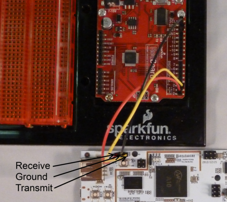
![Serial port pin mapping on the pcDuino]()
The A10 processor on the pcDuino has eight serial ports on board. Only two of these ports actually map to a Linux device: /dev/ttyS0 is the debugging port, and /dev/ttyS1 is the UART which is pinned out on the Arduino-ish header.
Pin mode settings
As mentioned on the GPIO page, the “mode” registers for each pin control the functionality of that pin. For serial I/O, you may need to write ‘3’ to the mode files for pins 0 and 1. The C++ code includes that; the serial library for Python does it by default.
Serial Communications in C++
Using C++ to access the serial port is not too hard. There are lots of good sites out there about serial port access in Linux; here’s a simple example program to get your started. All it does is configure the port, send “Hello, world!” across it, wait for an input keystroke to come back, then exit.
language:cpp
#include <stdlib.h>
#include <stdio.h>
#include <string.h>
#include <termios.h>
#include <unistd.h>
#include <fcntl.h>
#include "serial_test.h"

// Life is easier if we make a constant for our port name.
static const char* portName = "/dev/ttyS1";

int main(void)
{

  // The very first thing we need to do is make sure that the pins are set
  //   to SERIAL mode, rather than, say, GPIO mode.
  char path[256];

  for (int i = 0; i<=1; i++)
  {
    // Clear the path variable...
    memset(path,0,sizeof(path));
    // ...then assemble the path variable for the current pin mode file...
    sprintf(path, "%s%s%d", GPIO_MODE_PATH, GPIO_FILENAME, i);
    // ...and create a file descriptor...
    int pinMode = open(path, O_RDWR);
    // ...which we then use to set the pin mode to SERIAL...
    setPinMode(pinMode, SERIAL);
    // ...and then, close the pinMode file.
    close(pinMode);
  }

  int serialPort; // File descriptor for serial port
  struct termios portOptions; // struct to hold the port settings
  // Open the serial port as read/write, not as controlling terminal, and
  //   don't block the CPU if it takes too long to open the port.
  serialPort = open(portName, O_RDWR | O_NOCTTY | O_NDELAY );

  // Fetch the current port settings
  tcgetattr(serialPort, &portOptions);

  // Flush the port's buffers (in and out) before we start using it
  tcflush(serialPort, TCIOFLUSH);

  // Set the input and output baud rates
  cfsetispeed(&portOptions, B115200);
  cfsetospeed(&portOptions, B115200);

  // c_cflag contains a few important things- CLOCAL and CREAD, to prevent
  //   this program from "owning" the port and to enable receipt of data.
  //   Also, it holds the settings for number of data bits, parity, stop bits,
  //   and hardware flow control.
  portOptions.c_cflag |= CLOCAL;
  portOptions.c_cflag |= CREAD;
  // Set up the frame information.
  portOptions.c_cflag &= ~CSIZE; // clear frame size info
  portOptions.c_cflag |= CS8;    // 8 bit frames
  portOptions.c_cflag &= ~PARENB;// no parity
  portOptions.c_cflag &= ~CSTOPB;// one stop bit

  // Now that we've populated our options structure, let's push it back to the
  //   system.
  tcsetattr(serialPort, TCSANOW, &portOptions);

  // Flush the buffer one more time.
  tcflush(serialPort, TCIOFLUSH);

  // Let's write the canonical test string to the serial port.
  write(serialPort, "Hello, World!", 13);

  // Now, let's wait for an input from the serial port.
  fcntl(serialPort, F_SETFL, 0); // block until data comes in

  char dataIn = 0;
  do
  {
    read(serialPort,&dataIn,1);
  } while(dataIn == 0);

  printf("You entered: %c\n", dataIn);

  // Don't forget to close the port! Failing to do so can cause problems when
  //   attempting to execute code in another program.
  close(serialPort);
}

void setPinMode(int pinID, int mode)
{
  writeFile(pinID, mode);
}

// While it seems okay to only *read* the first value from the file, you
//   seemingly must write four bytes to the file to get the I/O setting to
//   work properly. This function does that.
void writeFile(int fileID, int value)
{
  char buffer[4];  // A place to build our four-byte string.
  memset((void *)buffer, 0, sizeof(buffer)); // clear the buffer out.
  sprintf(buffer, "%d", value);
  lseek(fileID, 0, SEEK_SET);   // Make sure we're at the top of the file!
  int res = write(fileID, buffer, sizeof(buffer));
}
Serial Communications in Python
Python requires an external library to use serial ports; however, it’s very easy to install. Just open up an LXTerm window and type
language:text
sudo apt-get install python-serial
Pyserial, the Python serial library, will be automatically installed.
Now, let’s run our first Python serial communications program. We’ll do the same thing we did in C++: open the port, wait for the user to input a keystroke, echo back the keystroke, then exit. Here’s the code:
language:python
#!/usr/bin/env python

import serial ## Load the serial library

## Select and configure the port
myPort = serial.Serial('/dev/ttyS1', 115200, timeout = 10)

## Dump some data out of the port
myPort.write("Hello, world!")

## Wait for data to come in- one byte, only
x = myPort.read()

## Echo the data to the command prompt
print "You entered " + x

## Close the port so other applications can use it.
myPort.close()
I2C Communications
I2C communication on the pcDuino is pretty easy.
Hardware
![I2C hardware resources on the pcDuino]()
As with serial communications, there are several I2C bus devices, but only one (/dev/i2c-2) is readily available to the user. A very, very important feature to take note of is that the I2C bus speed is fixed at 200kHz, which means that some devices may not work on the pcDuino I2C bus. The bus speed is fixed at driver compile time and cannot be changed from user space.
The pcDuino has on-board 2.2k pull-up resistors. These are pinned out to the Arduino-ish header, to the location typical for Arduino Uno R3 and later boards. On older boards, the pins were shared with analog inputs 4 and 5; there are solder jumpers on the pcDuino which allow you to redirect the SDA and SCL lines to those pins if you so desire. They’re labeled on the image above, and they’re designated R75 and R76.
There’s also a lovely set of tools that allow you to twiddle around with the I2C bus a bit without writing any code. To install this toolset, open a command line and type
language:text
sudo apt-get install i2c-tools
These tools can be a valuable sanity check for your hardware, so you can verify that problems you’re seeing are, in fact, in your code.
I2C Communications in C++
This simple program will connect to a couple of devices on the I2C port, read their device ID registers, and print them to the command line. The board used for the example is a SparkFun 6DOF Digital, but the principle is the same for any devices.
language:cpp
#include <stdlib.h>
#include <unistd.h>
#include <linux/i2c.h>
#include <linux/i2c-dev.h>
#include <sys/ioctl.h>
#include <fcntl.h>
#include <string.h>
#include <stdio.h>

int main(void)
{
  // Set up some variables that we'll use along the way
  char rxBuffer[32];  // receive buffer
  char txBuffer[32];  // transmit buffer
  int gyroAddress = 0x68; // gyro device address
  int xlAddress = 0x53;   // accelerometer device address
  int tenBitAddress = 0;  // is the device's address 10-bit? Usually not.
  int opResult = 0;   // for error checking of operations

  // Create a file descriptor for the I2C bus
  int i2cHandle = open("/dev/i2c-2", O_RDWR);

  // Tell the I2C peripheral that the device address is (or isn't) a 10-bit
  //   value. Most probably won't be.
  opResult = ioctl(i2cHandle, I2C_TENBIT, tenBitAddress);

  // Tell the I2C peripheral what the address of the device is. We're going to
  //   start out by talking to the gyro.
  opResult = ioctl(i2cHandle, I2C_SLAVE, gyroAddress);

  // Clear our buffers
  memset(rxBuffer, 0, sizeof(rxBuffer));
  memset(txBuffer, 0, sizeof(txBuffer));

  // The easiest way to access I2C devices is through the read/write
  //   commands. We're going to ask the gyro to read back its "WHO_AM_I"
  //   register, which contains the I2C address. The process is easy- write the
  //   desired address, the execute a read command.
  txBuffer[0] = 0x00; // This is the address we want to read from.
  opResult = write(i2cHandle, txBuffer, 1);
  if (opResult != 1) printf("No ACK bit!\n");
  opResult = read(i2cHandle, rxBuffer, 1);
  printf("Part ID: %d\n", (int)rxBuffer[0]); // should print 105

  // Next, we'll query the accelerometer using the same process- but first,
  //   we need to change the slave address!
  opResult = ioctl(i2cHandle, I2C_SLAVE, xlAddress);
  txBuffer[0] = 0x00;  // This is the address to read from.
  opResult = write(i2cHandle, txBuffer, 1);
  if (opResult != 1) printf("No ACK bit!\n");
  opResult = read(i2cHandle, rxBuffer, 1);
  printf("Part ID: %d\n", (int)rxBuffer[0]); // should print 229
}
I2C in Python
Python has a support package much like pySerial to make interfacing with I2C devices easier. To install it, open a command line and type
language:text
sudo apt-get install python-smbus
SMBus is the name given to the I2C derivative used on PC motherboards. The main differences are hardware-level and not reflected in the user coding level, so we’ll ignore them and just point out that the SMBus Python package can be used here.
This code does the same thing the C++ code does: queries the two devices on a 6DOF digital and prints the result to the command line.
language:python
#!/usr/bin/env python

import smbus

## As before, we'll create an alias for our addresses, just to make things
##   a bit easier and more readable later on.
gyroAddress = 0x68
xlAddress   = 0x53

## Initialize an smbus object. The parameter passed is the number of the I2C
##   bus; for the Arduino-ish headers on the pcDuino, it will be "2".
i2c = smbus.SMBus(2)

## With both of these devices, the first byte written specifies the address of
##   the register we want to read or write; for both devices, the device ID is
##   stored in location 0. Writing that address, than issuing a read, will
##   give us our answer.
i2c.write_byte(gyroAddress, 0)
print "Device ID: " + str(i2c.read_byte(gyroAddress)) ## should be 105

i2c.write_byte(xlAddress, 0)
print "Device ID: " + str(i2c.read_byte(xlAddress)) ## should be 229
SPI Communications
The pcDuino has headers exposing two different SPI buses. At this time, however, only one bus, and only one device on that bus, is supported. It’s possible to use other GPIO pins to add slave select lines, of course, with a hit to performance.
Hardware
![SPI pinout mapping on the pcDuino]()
The currently available SPI peripheral, SPI0, can be accessed through four of the pins on the Arduino-compatible headers along the bottom edge of the board. These pins break out the MOSI, MISO, SCK, and CS lines from the processor, allowing full hardware peripheral support of SPI communications.
SPI programming in C++
If you’ve been following along with the tutorial, a lot of this stuff should look familiar. Open a file descriptor for the spidev0.0 device, then use ioctl() to pass settings (defined in /linux/spi/spidev.h) to the peripheral. Actual message passing is a bit messy, though: you need to create a structure, then pass that structure to the file descriptor via ioctl().
We’ll be using the ADXL362 accelerometer breakout board as a test device in this code.
Don’t forget to use the pin mode files that we talked about back in the GPIO section to set the pins to SPI mode!
#include <stdio.h>
#include <unistd.h>
#include <fcntl.h>
#include <string.h>
#include <sys/ioctl.h>
#include <linux/spi/spidev.h>
#include "spi_test.h"

static const char *spi_name = "/dev/spidev0.0";

int main(void)
{
  int res = 0;  // We can use this to monitor the results of any operation.

  // The very first thing we need to do is make sure that the pins are set
  //   to SPI mode, rather than, say, GPIO mode.
  char path[256];

  for (int i = 10; i<=13; i++)
  {
    // Clear the path variable...
    memset(path,0,sizeof(path));
    // ...then assemble the path variable for the current pin mode file...
    sprintf(path, "%s%s%d", GPIO_MODE_PATH, GPIO_FILENAME, i);
    // ...and create a file descriptor...
    int pinMode = open(path, O_RDWR);
    // ...which we then use to set the pin mode to SPI...
    setPinMode(pinMode, SPI);
    // ...and then, close the pinMode file.
    close(pinMode);
  }

  // As usual, we begin the relationship by establishing a file object which
  //   points to the SPI device.
  int spiDev = open(spi_name, O_RDWR);

  // We'll want to configure our SPI hardware before we do anything else. To do
  //   this, we use the ioctl() function. Calls to this function take the form
  //   of a file descriptor, a "command", and a value. The returned value is
  //   always the result of the operation; pass it a pointer to receive a value
  //   requested from the SPI peripheral.

  // Start by setting the mode. If we wanted to *get* the mode, we could
  //   use SPI_IOC_RD_MODE instead. In general, the "WR" can be replaced by
  //   "RD" to fetch rather than write. Also note the somewhat awkward
  //   setting a variable rather than passing the constant. *All* data sent
  //   via ioctl() must be passed by reference!
  int mode = SPI_MODE0;
  ioctl(spiDev, SPI_IOC_WR_MODE, &mode);

  // The maximum speed of the SPI bus can be fetched. You'll find that, on the
  //  pcDuino, it's 12MHz.
  int maxSpeed = 0;
  ioctl(spiDev, SPI_IOC_RD_MAX_SPEED_HZ, &maxSpeed);
  printf("Max speed: %dHz\n", maxSpeed);

  // In rare cases, you may find that a device expects data least significant
  //   bit first; in that case, you'll need to set that up. Writing a 0
  //   indicates MSb first; anything else indicates LSb first.
  int lsb_setting = 0;
  ioctl(spiDev, SPI_IOC_WR_LSB_FIRST, &lsb_setting);

  // Some devices may require more than 8 bits of data per transfer word. The
  //   SPI_IOC_WR_BITS_PER_WORD command allows you to change this; the default,
  //   0, corresponds to 8 bits per word.
  int bits_per_word = 0;
  ioctl(spiDev, SPI_IOC_WR_BITS_PER_WORD, &bits_per_word);

  // Okay, now that we're all set up, we can start thinking about transferring
  //   data. This, too, is done through ioctl(); in this case, there's a special
  //   struct (spi_ioc_transfer) defined in spidev.h which holds the needful
  //   info for completing a transfer. Its members are:
  //    * tx_buf - a pointer to the data to be transferred
  //    * rx_buf - a pointer to storage for received data
  //    * len - length in bytes of tx and rx buffers
  //    * speed_hz - the clock speed, in Hz
  //    * delay_usecs - delay between last bit and deassertion of CS
  //    * bits_per_word - override global word length for this transfer
  //    * cs_change - strobe chip select between transfers?
  //    * pad - ??? leave it alone.

  // For this example, we'll be reading the address location of an ADXL362
  //   accelerometer, then writing a value to a register and reading it back.
  //   We'll do two transfers, for ease of data handling: the first will
  //   transfer the "read register" command (0x0B) and the address (0x02), the
  //   second will dump the response back into the same buffer.

  struct spi_ioc_transfer xfer;
  memset(&xfer, 0, sizeof(xfer));
  char dataBuffer[3];
  char rxBuffer[3];
  dataBuffer[0] = 0x0B;
  dataBuffer[1] = 0x02;
  dataBuffer[2] = 0x00;
  xfer.tx_buf = (unsigned long)dataBuffer;
  xfer.rx_buf = (unsigned long)rxBuffer;
  xfer.len = 3;
  xfer.speed_hz = 500000;
  xfer.cs_change = 1;
  xfer.bits_per_word = 8;
  res = ioctl(spiDev, SPI_IOC_MESSAGE(1), &xfer);
  printf("SPI result: %d\n", res);
  printf("Device ID: %d - %d - %d\n", rxBuffer[2], rxBuffer[1], rxBuffer[0]);
}

void setPinMode(int pinID, int mode)
{
  writeFile(pinID, mode);
}

// While it seems okay to only *read* the first value from the file, you
//   seemingly must write four bytes to the file to get the I/O setting to
//   work properly. This function does that.
void writeFile(int fileID, int value)
{
  char buffer[4];  // A place to build our four-byte string.
  memset((void *)buffer, 0, sizeof(buffer)); // clear the buffer out.
  sprintf(buffer, "%d", value);
  lseek(fileID, 0, SEEK_SET);   // Make sure we're at the top of the file!
  int res = write(fileID, buffer, sizeof(buffer));
}
SPI Programming in Python
Fortunately, a nice package exists for making SPI more accessible in Python. Unfortunately, installing it is difficult—much more so than the packages for I2C or serial. Here are the instructions to follow:
Update your package list for apt-get. In a terminal, type
sudo apt-get update
This will update the list of packages available to the apt-get program, ensuring that you get the right versions of the things we’ll be installing next.
Install git. Git is a source control tool used for version tracking, and it’s extremely useful. The SPI package in question resides on GitHub, which is a web portal for sharing git projects. To install git, pull up a terminal window and type
sudo apt-get install git
This installs the git toolchain; you don’t really need to know how to use it for what we’re doing here, but if you’re interested, we have a git tutorial that will teach you a lot of what you need to know.
Install python-dev. This is adds to python the ability to develop C-based extensions. To install, open a terminal window (or use the one that was open from installing git) and type
sudo apt-get install python-dev
Clone the SPI-Py git repository. This is the source code for the SPI python library we’ll be using. The command to type is
git clone https://github.com/lthiery/SPI-Py.git
Install the SPI-Py module. Type
 cd SPI-Py
 sudo python setup.py install
Now you’re set up and ready to write some code! Here’s a very simple Python app that will do essentially the same thing as the C++ code above does—connect to an ADXL362 and check the device ID register.
#!/usr/bin/env python

import spi

## The openSPI() function is where the SPI interface is configured. There are
##   three possible configuration options, and they all expect integer values:
##   speed - the clock speed in Hz
##   mode - the SPI mode (0, 1, 2, 3)
##   bits - the length of each word, in bits (defaults to 8, which is standard)
## It is also possible to pass a device name, but the default, spidev0.0, is
##   the only device currently supported by the pcDuino.

spi.openSPI(speed=1000000, mode=0)

## Data is sent as a tuple, so you can construct a tuple as long as you want
##   and the result will come back as a tuple of the same length.
print spi.transfer((0x0B, 0x02, 0x00))

## Finally, close the SPI connection. This is probably not necessary but it's
##   good practice.
spi.closeSPI()
learn.sparkfun.com |CC BY-SA 3.0
| SparkFun Electronics | Boulder, Colorado